The Lancet and USAID, Part Deux

It's actually worse this time

Some people complained that I did not properly steelman the Lancet paper concerning USAID cuts in my last poast about Cavalcanti et al. in The Lancet. Why did you use the all cause mortality instead of the causes of death that USAID focuses on? Why didn’t you use the controls they used? Who cares about Poisson regressions versus negative binomial regressions when children are dying?!

Some complaints were higher quality than others.

I took the complaining to mean people wanted more, so this is a shorter follow up poast addressing a few of the higher quality examples of such complaints. Because I think this paper is fundamentally flawed, I’ve also posted a condensed version of this post on pubpeer, but we’ll see if anything materializes there.

Disaggregated regressions

My original reproduction only regressed on all-cause mortality figures, not those causes of death that USAID explicitly focuses on preventing, those that make up the figure that I initially grew suspicious about.

This is a fair complaint. If you’re trying to measure USAID spend efficacy, people die from lots of things, and you should specifically measure the preventable deaths USAID might have had a hand in preventing.

Well, I should have done this initially, and I apologize, but the authors also think the analysis I did is relevant because they use all-cause mortality as well in several of their supplemental analyses. We’ll do the disaggregated analyses now and see if the effect size and significance changes. This is Figure 1 below.

Fig 1. RBA’s reproduction of Figure 1 in Cavalcanti et al., in green, with 2 other modeling choices.

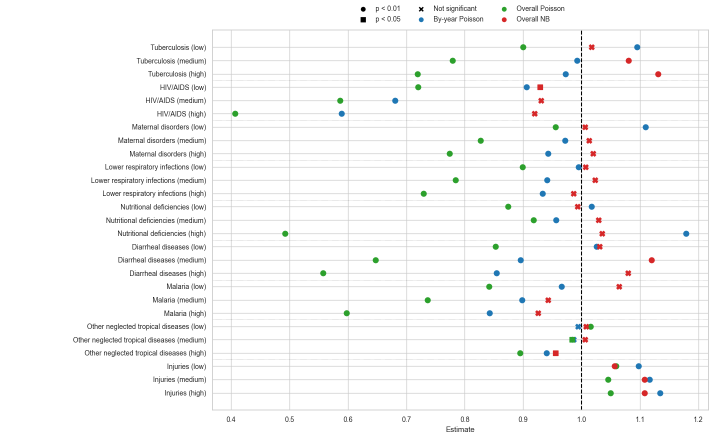
So the green dots are from the reproduction I attempted for each cause of death with no controls and the authors’ preferred Poisson spec. This does look a lot like their original figure, both from a significance and rate ratio size perspective. To take the most dramatic effect from Cavalcanti et al., the high USAID spend’s effect on HIV/AIDs deaths, they get a rate ratio of .35, while mine is .41; still a larger effect but in the same ball park without the massive number of controls they used.

I’m happy to call their figure successfully reproduced in green, and on these terms, I have no quarrel. Even the ordering effect (low spend effect < medium spend effect < high spend effect) mostly holds up except for one case (nutritional deficiencies).

The problems come in the blue and red dots. These are alternative models I tried both here in the disaggregated form and in Part 1. The blue dots are from a Poisson model with the spend quartilized by year and not over the entire dataset. I’ve gone back and forth on this, but overall think it’s a better choice. Look at the nutritional deficiencies plot high spend! They found a large negative impact (green) and I found a large positive impact (blue). What does this mean?

I think it means there’s reverse causation present in this data. USAID spends in response to a nutritional mortality crisis, so a famine causes increased USAID spend in a given year; the spend doesn’t effect the mortality as much. This might be the wrong way of thinking about it, and I’m happy to be corrected. I did do a few time-lagged comparisons to test for this, but they weren’t super persuasive, and if anything actually indicated there wasn’t a lot of reverse causation in here.

With the by-year binning (blue) strategy, you still get a ton of highly significant results even if the rate ratios are diminished compared to the green dots. This choice is a difference of opinion though.

The real problems which aren’t really differences of opinion come with the red dots, which are from negative binomial regressions I fit. The original all-cause mortality regression I did in Part 1 showed mild overdispersion in the the mortality statistics. This was Regression 4.

REGRESSION 4

ML estimation, family = Negative Binomial, Dep. Var.: all_cause_deaths
Observations: 2,393
Offset: log(population)
Fixed-effects: location_name: 129
Standard-errors: Clustered (location_name) 
                   Estimate Std. Error   z value Pr(>|z|) 
is_q2_overalltrue -0.019435   0.026313 -0.738613  0.46014 
is_q3_overalltrue  0.004617   0.035427  0.130325  0.89631 
is_q4_overalltrue -0.054367   0.040008 -1.358915  0.17417 
---
Signif. codes:  0 '***' 0.001 '**' 0.01 '*' 0.05 '.' 0.1 ' ' 1
Over-dispersion parameter: theta = 44.07691 

So the theta was 44. This indicates negative binomial might be a better choice over Poisson, but it’s a judgement call. When you do the disaggregated regressions, the problems can get much worse.

For Tuberculosis, the NB regression looks like this,

ML estimation, family = Negative Binomial, Dep. Var.: deaths
Observations: 2,387
Offset: log(population)
Fixed-effects: location_name: 128
Standard-errors: Clustered (location_name) 
                   Estimate Std. Error   z value Pr(>|z|)    
is_q2_overalltrue -0.134657   0.041458 -3.248041 0.001162 ** 
is_q3_overalltrue -0.060333   0.063335 -0.952590 0.340798    
is_q4_overalltrue -0.081167   0.066906 -1.213142 0.225076    
---
Signif. codes:  0 '***' 0.001 '**' 0.01 '*' 0.05 '.' 0.1 ' ' 1
Over-dispersion parameter: theta = 15.31242  
Log-Likelihood: -17,209.6   Adj. Pseudo R2: 0.238634
           BIC:  35,438.0     Squared Cor.: 0.954971

For HIV it looks like this

ML estimation, family = Negative Binomial, Dep. Var.: deaths
Observations: 2,372
Offset: log(population)
Fixed-effects: location_name: 127
Standard-errors: Clustered (location_name) 
                   Estimate Std. Error  z value Pr(>|z|)    
is_q2_overalltrue -0.165253   0.068308 -2.41922 0.015554 *  
is_q3_overalltrue -0.141972   0.094738 -1.49857 0.133986    
is_q4_overalltrue -0.226381   0.109644 -2.06470 0.038952 *  
---
Signif. codes:  0 '***' 0.001 '**' 0.01 '*' 0.05 '.' 0.1 ' ' 1
Over-dispersion parameter: theta = 7.08811  
Log-Likelihood: -16,648.1   Adj. Pseudo R2: 0.217525
           BIC:  34,306.5     Squared Cor.: 0.776309

And for Malaria, it looks like this

ML estimation, family = Negative Binomial, Dep. Var.: deaths
Observations: 1,704
Offset: log(population)
Fixed-effects: location_name: 87
Standard-errors: Clustered (location_name) 
                   Estimate Std. Error  z value Pr(>|z|)    
is_q2_overalltrue -0.265388   0.155586 -1.70573 0.088059 .  
is_q3_overalltrue -0.238676   0.182928 -1.30476 0.191976    
is_q4_overalltrue -0.461815   0.222806 -2.07273 0.038198 *  
---
Signif. codes:  0 '***' 0.001 '**' 0.01 '*' 0.05 '.' 0.1 ' ' 1
Over-dispersion parameter: theta = 1.466783  
Log-Likelihood: -12,300.9   Adj. Pseudo R2: 0.137927
           BIC:  25,271.5     Squared Cor.: 0.940756

In all cases the overdispersion gets much worse (look at the theta values) and the case for using negative binomial regression becomes much stronger. As you can see from these regression summaries and the red dots in Figure 1, the significance of USAID spend nearly disappears when you use negative binomial regression, even though it’s very clearly a better model choice.

The authors don’t agree. They defend the Poisson choice by saying the BIC is better and point to Web Table 12 in the supplemental material, Page 24.

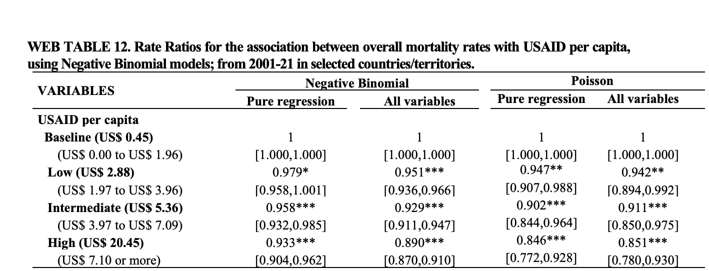
I simply don’t believe this table. Both from first principles and the reproduction I did, there’s absolutely no reason to suspect the significance and the rate ratios would be this similar for Poisson regressions and negative binomial regressions. It’s like saying the red dots and the green dots are very close together in Figure 1 above. It’s absurd.

But it gets worse when you look further down the page.

The information criteria for the Poisson regressions and the negative binomial regressions differ by 3 orders of magnitude! Why?

This initially confused me when I did it myself. The authors state the Poisson BIC is lower, and that’s why they picked it.

… to examine the stability of the results under different model specifications, we fitted Negative Binomial regression models and compared their Akaike Information Criterion (AIC) and Bayesian Information Criterion (BIC) values with those of the Poisson models (see Web Table 12). Although the Negative Binomial model is a generalization of the Poisson model and accounts for overdispersion, it also requires the estimation of an additional dispersion parameter, making it a less parsimonious alternative. In our case, the Poisson model yielded lower AIC and BIC values compared to the Negative Binomial model, indicating a better balance between model fit and complexity. Therefore, we retained the Poisson specification.

Well, it’s not just a bit lower, it’s hundreds of times lower, which should raise flags to any serious statistician. The problem is that they’ve fundamentally misunderstood the difference in likelihood functions between Poisson and negative binomial regressions; this difference makes the two BICs incomparable. The former uses a conditional fixed-effect likelihood and the latter does not. The correct way to judge which model family to use is to look at the overdispersion, and as I showed above, it strongly favors the negative binomial choice. A formal test of this on a Poisson model with no fixed effects using the HIV data concurs.

> dispersiontest(fresh_model, alternative = "greater")

	Overdispersion test

data:  fresh_model
z = 10.778, p-value < 2.2e-16
alternative hypothesis: true dispersion is greater than 1
sample estimates:
dispersion 
  57268.17

which suggests large overdispersion, and the Poisson model is therefore misspecified.

Unfortunately for the authors’ primary thesis, it means the red dots in Figure 1 are probably much more correct.

A few controls

A main comment this post received was on lesswrong, and suggested my reproduction was invalid because I didn’t use all the controls the authors did.

This is not a valid criticism. Controls are meant to eliminate the influence of confounding measurable elements in a regression analysis. They are not meant to be thrown into an analysis to improve the result with little thought to the causal mechanisms of what you’re modeling, and I’m sorry to report that’s what the authors did here. They state

These controls, combined with country fixed-effects models and other isolation factors, help refine the relationship between USAID per capita and changes in mortality over time.

The problem with this is that it’s not true. Some controls might work that way and others might not. But you can’t just state they’ll have this effect without thinking carefully about it, especially when you’re including more than a dozen of them.

Nevertheless, I did create the control variables the authors call “time shock” variables which correspond to mortality crises in certain years, and redo the regression analyses with and without them. The model spec here is now

\(\log(\mu_{it}) = \log(pop_{it}) + \sum_{q=0}^{3} \beta_q \, USAID_{qit} + \sum_{s=4}^{8} \beta_s \, T_y + \alpha_i + u_{it}\)

Here’s the HIV specific regression without them.

GLM estimation, family = poisson, Dep. Var.: deaths
Observations: 2,372
Offset: log(population)
Fixed-effects: location_name: 127
Standard-errors: Clustered (location_name) 
                   Estimate Std. Error  z value   Pr(>|z|)    
is_q2_overalltrue -0.328440   0.112825 -2.91107 3.6019e-03 ** 
is_q3_overalltrue -0.534091   0.200931 -2.65807 7.8588e-03 ** 
is_q4_overalltrue -0.899318   0.222045 -4.05015 5.1184e-05 ***
---
Signif. codes:  0 '***' 0.001 '**' 0.01 '*' 0.05 '.' 0.1 ' ' 1
Log-Likelihood: -2,422,286.0   Adj. Pseudo R2: 0.930509
           BIC:  4,845,582.3     Squared Cor.: 0.780087

and with them

GLM estimation, family = poisson, Dep. Var.: deaths
Observations: 2,372
Offset: log(population)
Fixed-effects: location_name: 127
Standard-errors: Clustered (location_name) 
                   Estimate Std. Error  z value   Pr(>|z|)    
is_q2_overalltrue -0.230366   0.088881 -2.59184 0.00954641 ** 
is_q3_overalltrue -0.353761   0.171012 -2.06863 0.03858068 *  
is_q4_overalltrue -0.588219   0.193735 -3.03621 0.00239576 ** 
y_2007true         0.191614   0.054471  3.51773 0.00043525 ***
y_2015true        -0.442836   0.048500 -9.13061  < 2.2e-16 ***
y_2019true        -0.660543   0.079945 -8.26245  < 2.2e-16 ***
y_2020true        -0.695461   0.081990 -8.48222  < 2.2e-16 ***
y_2021true        -0.800304   0.080319 -9.96404  < 2.2e-16 ***
---
Signif. codes:  0 '***' 0.001 '**' 0.01 '*' 0.05 '.' 0.1 ' ' 1
Log-Likelihood: -1,766,271.8   Adj. Pseudo R2: 0.949328
           BIC:  3,533,592.7     Squared Cor.: 0.846519

As expected, these controls diminish both the significance and the rate ratios for the USAID interventions. You can’t claim the analysis only works with the controls or improves with them. In most real world circumstances, it does not.

Coda

The control issue matters not so much, but the model misspecification is fatal for this paper, and personally I think it should be retracted. Both the retrospective regression analyses we’ve covered here and the Monte Carlo based projections we have not use the same mistaken Poisson specification. When this is corrected to use a negative binomial regression, the size of the rate ratios and the significances the authors find is very much undermined.